I learned a new word and it reminded me of Morse theory

Thalweg. Obviously German, built from thal, an outdated word meaning valley or dale, and weg, meaning way. So a thalweg is a "valley way," whatever that might mean.

But if you've ever taken a hike then you know exactly what it means: the path along the lowest part of the valley, which in principle should be the easiest path to take.

I came across this word while reading How to Read Water, by Tristan Gooley. He wasn't talking about valleys but rather about the other use of the word thalweg: the lowest part of the bed of a river, usually used as the official border between two states lying on either side of the river. If you don't think about it carefully, you might assume that the deepest part of a riverbed is in the center. If you are looking at a straight section you're probably right, but what happens in a bend of the river? The water is flowing because of gravity (otherwise you'd have a lake) and when there is a bend physics demands that the loose sediment on the bottom get pushed toward the outside of the curve. The result is that the thalweg runs closer to the outside bank in a bend; the river bed is steeper on that side and more gently sloped on the inside of the curve. Again, if you've ever looked closely at a clear, shallow river where you can see the bottom you might have noticed this. Here's a picture:

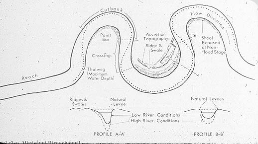
the dotted line is the thalweg.

There's math here, and the math I'm thinking of is Morse theory. Specifically, I'm thinking about parametrized families of smooth functions, which are well-understood thanks to a theorem of Cerf from 1970. That's a lot of words, so let me explain.

A smooth function \(f:M\to {\mathbb R}\) on a manifold \(M\) is Morse if all its critical points are nondegenerate. This means that the matrix of second partials is nonsingular at each critical point. Moreover, Sylvester's Law implies that the number of negative entries in any diagonalization of this symmetric matrix is the same; we call this number the index of the critical point. The prototypical examples of these are given by the functions \({\mathbb R}^2\to {\mathbb R}\) defined by \[ (x,y)\mapsto x^2+y^2 \quad (x,y) \mapsto -x^2+y^2 \quad (x,y)\mapsto -x^2-y^2\] 

The index of these maps is, respectively, 0, 1, and 2; geometrically they are a minimum, saddle point, and maximum, respectively. The Morse Lemma says that critical points of Morse functions all look like this; that is, there is a coordinate system centered at the critical point \(p\) of index \(i\) where the function has the form \(f(x) = f(p) - x_1^2-x_2^2-\cdots -x_i^2 + x_{i+1}^2+\cdots +x_n^2\). The existence of a Morse function on \(M\) (and there are lots of them) implies a lot about the topology of \(M\); this is a fascinating story, but not the one I have in mind here.

Say you have a smooth function \(f:M\to {\mathbb R}\) that isn't Morse. How not-Morse can it be? In isolation it can be pretty bad, but what Cerf was interested in was what can happen in a family of smooth maps on \(M\). Hopefully, you've come up with your favorite non-Morse function by now. It's \(f:{\mathbb R}\to {\mathbb R}\) defined by \(f(x) = x^3\), right? You can generalize this to any Euclidean space by taking this map in the first coordinate and then a sum of quadratics in the others: \(f(x) = \pm x_1^3 - x_2^2 - \cdots -x_i^2 + x_{i+1}^2 + \cdots + x_n^2\). The critical point at the origin is degenerate, but only because we've cubed the first coordinate.

So now let's think about a family of smooth maps \(F:M\times [0,1]\to {\mathbb R}\). This means that (a) each \(F(-,t)\) is a smooth map on \(M\), and (b) the assignment \(F\) is a smooth map on the manifold (with boundary) \(M\times [0,1]\). There are lots of questions we might ask. The first is if it is possible for each \(F(-,t)\) to be a Morse function. This is certainly possible: take the constant family \(F(x,t) = f(x)\) determined by a single Morse function \(f:M\to {\mathbb R}\). This is not very interesting. However, Morse functions are generic on a given manifold. That is, given any smooth map on \(M\), there is a Morse function arbitrarily close by. So we might then turn to the more interesting question of just how not-Morse functions in the family can be. And this is where Cerf's work comes in.

The executive summary is this: Suppose you have a family of smooth functions \(F(-,t)\) where \(F(-,0)\) and \(F(-,1)\) are Morse. Then Cerf proved that there is another family \(G(-,t)\), arbitrarily close to \(F(-,t)\) such that each \(G(-,t)\) is Morse except for finitely many values of \(t\in [0,1]\). At those values, there is a single degenerate critical point \(p\) in \(M\), and there are coordinates around it so that \(G(x,t) = c + x_1^3 +\epsilon_2 x_2^2 +\cdots + \epsilon_n x_n^2\) where \(\epsilon_j\in\{\pm 1\}\). So, if you're willing to wiggle your family just a little bit you get Morse functions almost everywhere and where you don't you just get a cubic singularity. The whole story is richer than this, of course, and involves birth-death points and bifurcation diagrams. That's another post, though.

What does all this have to do with the thalweg? You have to take the right point of view first. Thinking of the riverbed as the depth function over some 2-dimensional patch of the earth is not especially illuminating. Most of the time you won't have any critical points since the riverbed gently slopes downstream. Sure, there are pools that form in rivers where there are depressions in the bed, but those are not part of the thalweg as a rule. No, the proper thing to do here is to consider cross-sections of the riverbed as graphs of a function on an interval (the width of the river). Like this:

a cross-section of the river

Here we have a function on some interval and using standard calculus we can find its local extrema. We then think of the riverbed as the graph of a family of these cross-sections \(F:I\times L\to {\mathbb R}\), where \(I\) is an interval of length equal to the maximum width of the river and \(L\) is an interval of the form \([0,\ell]\) where \(\ell\) is the length of the river. For each \(t\in L\), let \(X_t\) denote the finite collection of local minima for \(F(-,t)\). The locus of points \(\{(x,t): x\in X_t, t\in L\}\) will have possibly many connected components, but it will contain one component \(T\) extending the length of the river; \(T\) is the thalweg. The other components will correspond to places where a ridge may arise in the riverbed, leading to a stretch of local minima that eventually merge back with the minima in \(T\). This corresponds to what goes on in Cerf theory--new critical points may be born, some may die.

This is all just an approximation, of course. While most of these cross-sections will be the graphs of smooth maps, there will be some that aren't. And riverbeds shift all the time, so it's not like the thalweg is a static thing. Indeed, it would be interesting to let these cross-sections vary in time and track the evolution of the thalweg. Floods and seismic events can certainly move it around.

Anyway, I like this word, thalweg, and I really like the math it made me think of.